There are multiple sources of power loss in antenna systems — ohmic losses in the antenna conductors themselves and dielectric losses in coaxial cables and PCB materials are probably the two most common sources of loss. Its unlikely that many antenna engineers these days have ever had to contend with an oak tree or juniper bush sucking power from their transmitting antenna, however such problems really do exist! At low frequencies where transmitting antennas can get quite large, the presence of vegetation around the antenna structure can result in power loss and a subsequent degradation in antenna performance.
The first part of my career as an engineer was spent in Civil Service — I was a VLF (very low frequency) antenna engineer in the Submarine Broadcast Systems Division at a large Navy electronics laboratory in California. Very low frequency radio signals are used by numerous Navies around the world to communicate with their fleet of submerged submarines. As it turns out, radio signals in the frequency range of 20 kHz to 60 kHz can penetrate seawater to a depth of several tens of meters. A submarine typically drags a long wire antenna behind it which streams along just below the surface, allowing the radio signals to be received. The trouble with using VLF radio signals for communication is their long wavelength — at 20 kHz an electromagnetic wave has a wavelength of 15 kilometers, and radio transmitting antennas generally need to be at least one-quarter wavelength long in order to function efficiently. As such, a quarter-wavelength antenna at 20 kHz is impossible to build. Most VLF transmitting sites in use today employ transmitters in the 20 kHz to 40 kHz range that generate powers as high as 1 megawatt, and use antenna systems comprised of multiple towers over 1000 feet in height. Capacitive top-loading for these antennas frequently incorporate grids of wire thousands of feet long that are suspended in the air by additional towers and spanning tens of acres of real estate.
Despite their tremendous physical size, VLF transmitting antennas are electrically very small, that is, their overall physical dimensions are significantly less than one wavelength at their operating frequency. This makes a VLF antenna very similar to one of those small surface mount chip antennas you often find on printed circuit boards that are used for Bluetooth or WiFi. Anyone who has designed with these types of surface mount PCB antennas knows that they are very inefficient — the placement of these antennas on a PCB must be done with care, as any objects in close proximity to the antenna (other components, ground planes, connectors, etc.) can significantly degrade their performance, reducing their efficiency even further.
The same problem exists with VLF antennas — it is not uncommon to find VLF transmitting antennas in operation today that have efficiencies below 30%. As many of these transmitting systems are required to radiate many hundreds of kilowatts, any small degradation in antenna performance can result in very large increases to the electric bill each month! As such, anything that can be done to mitigate power losses that occur in VLF antenna systems has the potential to reduce the overall operating cost of the facility.
The photo below is an aerial shot of the U.S. Navy’s VLF transmitting facility at Jim Creek, Washington. This radio facility has been in operation since 1952 and operates on a frequency of 24.8 kHz:
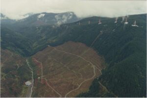
This antenna is known as a “valley span” antenna — multiple wires are strung across the valley and supported by towers along the ridges on either side. These wire catenaries are each over one mile in length and form the capacitive top-loading for the antenna system. At the center of each catenary a vertical downlead extends to nearly the valley floor, and then travels along a series of short supporting towers to the main transmitter building located at the center of the valley. The entire antenna system has the appearance of a gigantic hair net suspended from towers on each ridge. Notice that the foliage across most of the valley has been removed — this clear-cutting of foliage is intentional and is meant to reduce the power losses in the antenna system. When the Jim Creek transmitter first went into operation, it was observed that the radiated power of the antenna system was somewhat higher in winter than in summer. It was found that these differences were a result of power loss occurring in the foliage growing in the valley underneath the antenna system (Watt, A.D., VLF Radio Engineering, Pergamon Press, New York, 1967, pp.149-153). As I have already stated, anything which degrades the efficiency of an antenna like this contributes to a significant increase in the cost of electricity to operate the station.
How can one actually measure the power loss in the foliage across an entire valley like this? Well — back in 1991 I had the opportunity to do just that! My team of engineers was assigned the job of estimating the power loss in the entire antenna system due to the foliage in the Jim Creek valley and providing a measurement report to the U.S. Navy. To accomplish this task, we constructed a “Frankenstein-looking” apparatus out of a bunch of chicken wire and 4×4 lumber:
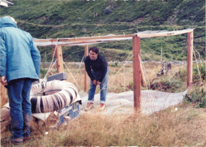
That’s me — standing in the middle of what is actually a parallel-plate capacitor. The top and bottom plates are fabricated from chicken wire and supported by the 4×4 lumber. Immediately to the left of me in the photo is a large toroid — Litz wire wound around a large truck tire inner tube (for those of you that have never heard of Litz wire, take a look here). The toroid and chicken wire capacitor are connected in series, forming a tuned circuit. A capacitance decade box, also visible directly above the toroid, is connected in parallel with the chicken wire capacitor so its overall value can be adjusted so the entire tuned circuit is resonant at 24.8 kHz (the operating frequency of the Jim Creek transmitter). Our source of RF energy was a Hewlett-Packard signal generator driving a 100 watt commercial amplifier.
So — how does this work? Our team spent some time scouting around the valley beneath the antenna to see the kinds of vegetation present, and we identified several “garden variety” shrubs. After choosing a specific shrub for testing, we assembled the chicken wire capacitor so that the shrub was situated at the center of the bottom capacitor plate and protruding up into the space between the plates. In order to make this assembly process easier, the bottom plate of the capacitor was made from two sections of chicken wire each with a semicircular notch cut into one edge. When placed together, the two notches formed a circular hole which surrounded the base of the shrub. The two halves of the chicken wire were then connected together with a bunch of alligator clips to ensure electrical continuity. This tuned circuit, which now included the effects of the shrub, was energized with 24.8 kHz RF energy. The capacitance decade box settings were then varied until the entire tuned circuit resonated at 24.8 kHz. Our method of detecting resonance was simple, but extremely cool — using a two-channel oscilloscope, we connected one channel across the amplifier output in order to monitor the tuned circuit voltage. The other scope channel was connected to a current probe that monitored the current flowing in the tuned circuit. By placing the oscilloscope display into X-Y mode, the voltage and current waveforms combine and appear on the scope as an ellipse (the voltage and current are out of phase with each other) — for those of you old enough to remember, this is known as a Lissajous Figure. Adjusting the capacitance decade box so that the ellipse collapses to a straight line indicates that the voltage and current are in phase — resonance has been achieved!
Now that the tuned circuit is resonant, the next step is to measure the circuit’s bandwidth. Noting the value of the current at resonance, the frequency of the signal generator is varied both above and below 24.8 kHz to observe the frequencies at which the current drops to 0.7071 times its value at the resonant point (this is the 3dB point on the resonance curve). Taking the difference between the high frequency and the low frequency yields the bandwidth of the tuned circuit. With the bandwidth determined, the next step in the measurement is accomplished with a bucksaw and a set of pruning shears — the entire shrub is cut up and completely removed from the chicken wire capacitor, and the bandwidth measurement is repeated. With the shrub no longer present, the total loss in the tuned circuit decreases, subsequently decreasing the bandwidth of the circuit. By looking at the change in bandwidth between the two configurations, the “equivalent series resistance” of the shrub is determined. Since the current flow in the tuned circuit is known, the power loss in the shrub is determined.
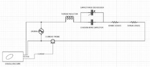
The diagram above is the schematic diagram for the test setup that we used. The shrub appears in the circuit as a resistance along with the other ohmic resistance that is present in the circuit (mostly the resistance of the Litz wire in the toroid, but there is also some resistance in the wiring and miscellaneous connectors used in the setup). What follows is the math used to extract the equivalent series resistance of the shrub.
When the shrub is part of the circuit, the “Q” of the tuned circuit at resonance is given by:
Q_{shrub} = \frac{2\pi f_0 L}{(R_{loss} + R_{shrub})}Once the shrub is removed, its equivalent series resistance is no longer present, so the expression for the “Q” at resonance becomes:
Q_{noshrub} = \frac{2\pi f_0 L}{R_{loss}}The “Q” of a tuned circuit is inversely proportional to its bandwidth — another way to express the “Q” of a tuned circuit is like this:
Q = \frac{f_0}{\Delta f} = \frac{f_0}{BW}Using this definition, we get a pair of equations:
\begin{aligned} BW_{shrub}& = \frac{R_{loss} + R_{shrub}}{2 \pi L}\\ BW_{noshrub}& = \frac{R_{loss}}{2 \pi L} \end{aligned}Solving these for the equivalent series resistance of the shrub:
R_{shrub} = 2 \pi L (BW_{shrub} - BW_{noshrub})Notice that the inductance of the inner tube toroid needs to be known — we measured the inductance of the toroid in the lab, so this was a known quantity.
So far, so good — but how does this relate to the power dissipated by a shrub when it is sitting on the valley floor under the antenna? We’ve computed an equivalent series resistance for the shrub, and we can compute the power it dissipates by utilizing the current flow in the tuned circuit at resonance:
P_{shrub} = I^{2} R_{shrub}How do we use this resistance when we consider the entirety of the foliage that sits beneath the antenna? The answer may surprise you — we actually don’t use this resistance at all! We introduced the idea of an equivalent series resistance of the shrub solely to permit us to compute the power dissipated by a single shrub. With the actual dissipated power known to us, the next step in unraveling this measurement for the entire valley beneath the antenna is realizing that the power dissipation that occurs in the shrub is a direct consequence of it being immersed in the electric field of the antenna system! If we can measure the electric field that exists inside the chicken wire capacitor around the shrub, we can establish a relationship between the power dissipation in the shrub as a function of the surrounding electric field.
Fortunately, in order to get at the value of the electric field inside the chicken wire capacitor we don’t need to measure it directly. At VLF, the electric field inside the chicken wire capacitor is so slowly varying in time that it can be treated as a static DC electric field. Even more important, so long as we only consider the behavior of the field near the vertical axis of the capacitor (we stay away from the edges of the chicken wire), the electric field is nearly uniform (that is, its value does not change with position). Using this very-good assumption (once again, at VLF this works!), the electric field inside the chicken wire capacitor where the shrub is located is just equal to the voltage across the capacitor divided by the spacing between the top and bottom plate:
E = \frac{V_{capacitor}}{d_{plates}}During our measurements, we did not directly measure the voltage across the capacitor — we don’t need to make this measurement, as we have already measured the bandwidth of the circuit when the shrub was present inside the chicken wire capacitor. How are these two quantities related? It turns out that, for a series resonant circuit, the voltages across the individual reactances at resonance are equal to each other (although they are 180 degrees out of phase) and have a magnitude equal to:
V_{peak} = Q V_{in}where V_in is the input voltage across the entire tuned circuit. Making a few substitutions, the expression for the voltage across the capacitor is:
V_{peak} = \frac{f_0}{BW_{shrub}}V_{in}It is a good thing we don’t need to measure this voltage directly — it is in the ballpark of several thousand volts! However, with this information at hand, the magnitude of the electric field inside the chicken wire capacitor is known to a good degree of approximation, giving us a relation between the power lost in the shrub when it is immersed in an electric field equal to that inside the capacitor. Estimating the power loss for any other electric field strength is made by noting that the power absorption by a conductor immersed in an electric field is proportional to the square of the electric field strength. When the Jim Creek radio facility is transmitting, the electric field on the valley floor is easily measured with standard field strength equipment, and the resulting field map is overlaid on a topographic chart.
The last step in the entire process of measuring power loss from shrubbery was perhaps the most difficult — we needed to count the shrubs! Here again, the use of a good approximation tool came in handy — we picked out a number of areas around the valley approximately 50 feet by 50 feet in size, and walked these areas while counting the shrubs. The areas we chose were based on how uniform they looked to the human eye as well as where in the valley they were located. Extrapolating this information out to the entire valley using photographic data allowed us, at long last, to arrive at a power loss estimate due to shrubbery residing in the valley.
How accurate were our measurements? When dealing with an antenna as large as the Jim Creek antenna, there are so many variables that contribute to the total power loss it is nearly impossible to get an answer with an accuracy better than 25% to 30%. As part of our measurement work we had the advantage of being able to review power loss data taken throughout the history of the station’s operation. The primary objective of our measurement effort was not so much to determine the actual power loss at a high level of absolute accuracy as it was to determine that no significant changes to the antenna system power loss had taken place. This knowledge is valuable from the standpoint of establishing an overall trend in antenna performance — this information is invaluable for predictive maintenance purposes.
A final comment about that picture of me inside the chicken wire capacitor — one of the perks of this job was my entire team got the opportunity to have our loss resistance at 24.8 kHz directly measured. The photo was my turn in the capacitor — I don’t remember what my loss resistance was, but I was sure to keep my head down, otherwise I would have burned the hair off the top of my head if it touched the top plate.
Until next time,
David
Recent Comments